The COVID-19 pandemic has interrupted the day-to-day life of all Sri Lankans. At the time of writing, the entire country is in lockdown. As of now, due to strict interventions, the disease spread seems to have slowed down. However, it is not completely clear what we should expect in the future, especially when interventions change. To shed some light, we have developed an interactive tool to model the spread of COVID-19 in Sri Lanka using a classical SEIR (Susceptible → Exposed → Infected → Removed (i.e recovered and fatal) infectious disease model. We also modified the model to account for the Sri Lankan setting.

In our model, the entire population is divided into the following classes:

• \(S\) - Susceptible individuals
• \(E_0\) - Exposed individuals before they become infectious
• \(E_1\) - Exposed individuals after they are infectious
• \(I_0\) - Asymptomatic individuals
• \(I_1\) - Infected individuals with mild symptoms
• \(I_2\) - Infected individuals with severe symptoms (require hospitalization)
• \(I_3\) - Infected individuals at critical stage (require ICU admission)
• \(R\) - Recovered individuals
• \(D\) - Fatalities

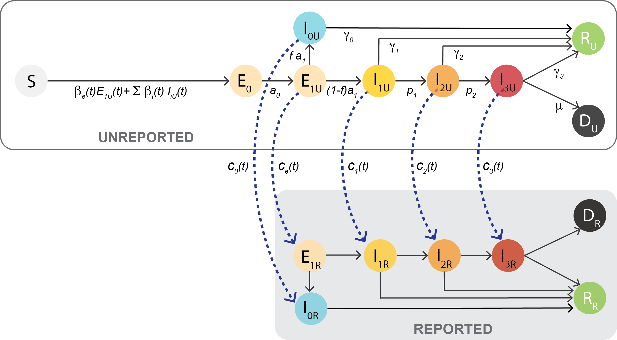
Susceptible (\(S\)) individuals contract the disease from infected individuals in the classes \(E_1, I_0, I_1, I_2,\) and \(I_3\). They then move to the exposed class (\(E_0\)). After an incubation period (~3 days) in \(E_0\), they become infectious in the \(E_1\) class, and stay in the infectious-exposed class \(E_1\) for ~2 days. From \(E_1\), they can either move to an asymptomatic class, \(I_0\), or to the mild symptomatic class, \(I_1\). The percentage of asymptomatic vs. symptomatic individuals is captured by the fraction \(f\), and is assumed to be 0.3 (i.e. 30% are asymptomatic). The classes \(E_1, I_0, I_1, I_2,\) and \(I_3\) are further decomposed into two categories: reported and unreported (e.g. \(E_{1R}\) and \(E_{1U}\)). The ratio between the number of reported and unreported individuals in each of these classes is controlled by the time-varying parameters \(c_e(t), c_0(t), c_1(t), c_2(t), c_3(t)\). Each \(c(t)\) fraction represents the percentage of unreported cases that get reported/diagnosed on a given day.

According to literature, roughly 81% of the symptomatic individuals (in \(I_1\)) recover after mild symptoms (in ~6 days) and move to the recovered class (\(R\)). The remaining 19% from \(I_1\) develop severe symptoms and move to the \(I_2\) class. These severe cases require hospitalization. About three-fourths from \(I_2\) recover after hospitalization (in ~4 days), but the remaining one-fourth develop critical symptoms and require ICU treatment. About 40% of the critical cases are fatal and the rest recover after ICU treatment (in ~10 days). These numbers were derived from the published literature of the COVID-19 spread in China, and were used to calculate the rate parameters, \(a_0, a_1, f, \gamma_0, \gamma_1, \gamma_2, \gamma_3, p_1, p_2,\) and \(\mu\).

Next, we had a significant number of infected individuals (tested positive) who entered the country from abroad, but were strictly quarantined before they could infect others. We assumed that all these cases enter the country at the mildly-infected stage (\(I_{1R}\)), although it is possible that they enter during the exposed period as well. When we run the model, we add these cases to the population based on the date they tested positive.

Governing equations

The system of coupled differential equations that model the evolution of the number of individuals in each of the 16 classes (with sub-categories) is given by: $$ \begin{align} \dot{S} &= -\left( \beta_e E_{1U} + \beta_0 I_{0U} + \beta_1 I_{1U} + \beta_2 I_{2U} + \beta_3 I_{3U} \right) S \\ \dot{E}_0 &= \left( \beta_e E_{1U} + \beta_0 I_{0U} + \beta_1 I_{1U} + \beta_2 I_{2U} + \beta_3 I_{3U} \right) S - a_0 E_0 \\[1em] \dot{E}_{1U} &= a_0 E_0 - a_1 E_{1U} - r_e(t) \\ \dot{I}_{0U} &= f a_1 E_{1U} - \gamma_0 I_{0U} - r_0(t) \\ \dot{I}_{1U} &= (1-f) a_1 E_{1U} - (\gamma_1 + p_1) I_{1U} - r_1(t) \\ \dot{I}_{2U} &= p_1 I_{1U} - (\gamma_2 + p_2) I_{2U} - r_2(t) \\ \dot{I}_{3U} &= p_2 I_{2U} - (\gamma_3 + \mu) I_{3U} - r_3(t) \\ \dot{R}_{U} &= \gamma_1 I_{1U} + \gamma_2 I_{2U} + \gamma_3 I_{3U} \\ \dot{D}_{U} &= \mu I_{3U} \\[1em] \dot{E}_{1R} &= -a_1 E_{1R} + r_e(t) \\ \dot{I}_{0R} &= f a_1 E_{1R} - \gamma_0 I_{0R} + r_0(t) \\ \dot{I}_{1R} &= (1-f) a_1 E_{1R} - (\gamma_1 + p_1) I_{1R} + r_1(t) + q_{entry}(t) \\ \dot{I}_{2R} &= p_1 I_{1R} - (\gamma_2 + p_2) I_{2R} + r_2(t) \\ \dot{I}_{3R} &= p_2 I_{2R} - (\gamma_3 + \mu) I_{3R} + r_3(t) \\ \dot{R}_{R} &= \gamma_1 I_{1R} + \gamma_2 I_{2R} + \gamma_3 I_{3R} \\ \dot{D}_{R} &= \mu I_{3R} \end{align} $$ The time-varying functions \(r_e(t), r_0(t), r_1(t), r_2(t),\) and \(r_3(t)\) simulate the act of "reporting" by transferring individuals from the unreported classes to the reported classes, based on the corresponding daily reporting fractions \(c_e(t), c_0(t)\) etc.